Rudiments of Geometry and Topology for Computational Design

Introduction

This is a very short introduction for impatient Computational Design practitioners. Geometry and Topology are two distinct branches of mathematics:

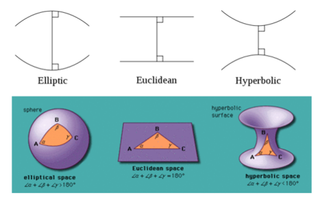
• Geometry: Geometry is the study of metric properties of shapes such as distances, lengths and angles. The field of geometry has most probably started because of interests in surveying lands (e.g. for taxation purposes) on Earth and as such the name geometry comes from the Greek words Geos (Earth) and Metria (measurement) Γεωμετρία. Nowadays, geometry as the study of shapes goes beyond such applications and tends to be much more abstract. As you might have guessed or heard, the field of geometry is quite old, probably the oldest branch of mathematics after arithmetic, dating back to Ancient Greece and Ancient Egypt (around 6th century B.C.). Geometric constructions specially those based on simple rule and compass geometry constructs have had a long history in architecture due to their intuitiveness and their applicability in masonry. As such, for most people the very term geometry is associated with that kind of geometry, especially when mentioned in conjunction with the term architecture. However, such forms of geometry are mainly limited to Euclidean geometry, while Non-Euclidean geometries such as elliptic or hyperbolic geometry naturally arise in computational design, e.g. in dynamic-relaxation, i.e. generation of non-bending structures, namely [eliptic] compression-only catenary/funicular structures and [hyperbolic] tension-only soap-films/minimal surfaces structures.

• Topology: In contrast, however, the field of topology is much younger, dating back to the seminal works of Euler on incepting graph theory and the study of polyhedral tesselations (in the 18th century A.D.). The cope of topology is the study of the so-called topological invarianats such as connectedness, continuity, closedness and dimension which remain unchanged during the so-called topological transformations. Contrary to what the name suggests, topological transofrmations are those transformations that do NOT alter the topology of the set/shape under transformation. Anyhow, the field called topology (again the name is consisted of two Greek words τόπος, ‘place, location’, and λόγος, ‘study’) has developed much beyond the study of such invariants in shapes and become a very abstract field of study concerned with sets and algebraic constructs. Topology tends to be an elusive subject of study, whose definition even baffles experienced mathemataicians. Even though it looks like that the field is about some cool objects that could be the subject of pub quizzes (the Möbius strip, the Klein bottle, etc.) there is much more abstract matters that need to be understood before being able to enjoy such discussions.

  

  This image, and some of the definitions loosely given above can be traced to here.

• Computer Graphics: Before getting into details of these, it is important to note that our point of departure in our journey for getting introduced to these two subject areas starts from the field of Computer Graphics that is much younger (dating back to 1960’s).

• Computational Design:Computational Design is an umbrella term referring to the research, development, and utilization of processes for systematically designing the configuration (topology) and shape (geometry) of objects such that they fulfill or optimally achieve certain functional requirements. Due to the focus of this lecture on computational design, both geometry and topology are re-introduced in a computational context. Luckily, since the objects of interest in computational design have visible shapes we hope that this introduction remains intuitive. A basic understanding of digital computers and representation of compound objects in them is essential for following this lecture. Therefore, the reader is recommended to review the subjects covered in the previous lecture on the Rudiments of Linear Algebra and Computer Graphics.

Re-introduction

The reasons I call this section re-introduction are twofold, I would like to:

1. Emphesise that our primary object of study (and design) is not shapes but spaces; and in doing so, i.e. shifting focus from shapes to spaces,
2. Give a glimpse of the generality of geometry and topology beyond low-dimensional and visible applications. This is only important for those who may wish to continue reading more about Machine Learning and Artificial Intelligence.

Before shifting gears towards understanding the meaning of space, we also need to comprehend the meaning of a frequently abused word: ‘model’.

• What is a model?: By using the word model (apart from people modelling for fashion) we often mean to refer to a replica of something real, albeit not represnting its entirty but replicating some of its features with various degrees and kinds of abstractions. In the context of architeture and design models are often geometric models sometimes built physically. In addition to these geometric models there are other kinds of mathematical models and computational models geared towards mathematical analysis or computational simulation for studying the natural properties, functionality, and dynamics of systems and phenomena.
• What is a spatial model?: A particular type of such models are concerned with space, phenomena embedded in space, or objects whose spatial form or distribution are non-trivial. Such models are of key interest to the fields of Computer Graphics, Computer-Aided-Design, Geographical-Spatial Information Sicence (a.k.a. GI-Science) and alike. We colloquially refer to these models as models of space or spatial models. A key factor in categorization of models of any kind is their representation and abstraction framework. A classification of spatial models, from the most concrete (Geographical Models of Space) to Geometric and topological models and beyond is presented in this paper.

While most of these matters may seem quite pedantic and unrelated to the main subject here, I find it important to present the main subject in a general context. Particularly, it is important to present this context to argue why it is important to go beyond learning geometry and understand topology.

Space and Dimensionality

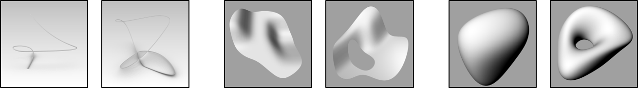
Apart from shallow daily encounters with the terms space and dimensionality, and apart from all the interesting science fiction stuff like going beyond this dimension and entering another dimension, or the popular science articles about time as being the fourth dimension and all that, it is important to understand what they mean mathematically if we want to feel good in the rest of the journey towards understanding computer geometry and topology! Not convinced yet? Let us begin with a dilemma then: what is the dimensionality of the following objects?

Are these objects not three dimensional? Yes, because they are all drawn in a 3D space and their ‘points’ do have three non-zero coordinates. However, at the same time, you could/should agree that there is something one-dimensional about the objects on the left, something two-dimensional about the objects in the middle, and something three-dimensional about the objects on the right. To be clear, let us change the focus from the space in which these objects are drawn to the space they confine within themselves. The former is called the embedding space and the latter is the embedded space. Well, the simplest way I can define dimensionality in an intuitive way is to first distinguish geometrical and topological dimensionality:

• geometrical dimensionality: the dimensionality of the vectors representing the points/vertices of the objects
• topological dimensionality: the dimensionality of the space confined within the objects, i.e. the number of possible directions of movement within the object, which is only meaningful if the object in question remains ‘everywhere locally similar to’ a simple space of the same dimension (i.e. a Euclidean space of the same dimension)

Thus, in other words, these objects can be at the same time 3D objects from a geometrical point of view while they are 1D, 2D and 3D from left to right, from a topological point of view. Well, so far, this is a mathematical discussion. Note that we implicitly assumed that in a space you can move from anywhere you are to another location continuously from where you are to wherever the other location may be. This very possibility of movement is in fact what distinguishes a space from a bunch of locations. We shall later see that this is because of ‘a topology’ (as a single object, the same way we may refer to ‘a geometry’) defined on that bunch of (set of) locations.

Recall that I mentioned above the local similarity to a Euclidean space (named in the honour of Euclid)? If you do not feel comfortable with the idea of Euclidean space, its dimensionality, and its connection to the Cartesian product (named in the honour of René Descartes), I would suggest reading the previous lecture notes on Linear Algebra (the section called dimensionality). In that lecture I preached a lot about the intuition behind this notion of dimensionality, and so here I should make it a little more pedantic to prepare you for the next subjects. The idea of local similarity in mathematical terms is called homeomorphism and it concerns the similarity of the so-called tangent-space at a location on a manifold with a Euclidean space of some dimension. Well, in plain English, when standing on a giant 3D object with a smooth and planar surface (at least as planars as you can see) then it feels convenient to assume that the object is locally similar to a 2D plane, and so, it probably would not hurt you if I recapitulated the definitions of low-dimensional manifolds from the previous lecture:

• 0-Manifold: a Point (the space therein everywhere resembles a 0-dimensional Euclidean Space)
• 1-Manifold: a Curve (the space therein everywhere resembles a 1-dimensional Euclidean Space)
• 2-Manifold: a Surface (the space therein everywhere resembles a 2-dimensional Euclidean Space)
• 3-Manifold: a Solid (the space therein everywhere resembles a 3-dimensional Euclidean Space)

Note that from now on we focus our attention on manifold objects (without loss of generality) because of many nice properties that are brought about by manifoldness, especially that we can refer to objects with their topological dimensionality, i.e. the object in question has the same dimensionality respectively all over its domain and range. What is a domain and what is a range? Well, in the language of calculus, the domain of a ‘function’ is the interval or the region from which the function takes its inputs. Similarly, the range of a function is the interval or the region to which the function in question ‘maps’ the inputs. With reference to these two notions, a k-manifold (curve, surface, or hyper-surface) is a ‘smooth’ map (range) of a function from a k-dimensional domain. Alright, now let us shift gears from mathematics to computer science, accepting that whatever we represent in computers must be eventually representable in terms of the simplest units of information or bits.

Digital Computing versus Analog Computing

Perhaps the best intuitive example for digital versus analog production of data is the Piano versus the Violin. Can you see why I think the telegraph is more modern than the telephone?

1. Analog Computing: If you studied engineering some 40-70 years ago at a prestigious university of technology, you would have to pass a fantastic, tough, and scary course called analog computing or something like that (analogue is also an alternative dictation). Although the words analog and digital have strong electronics-related connotations, an Analog Computer can be conceptualized as a machine (which could be mechanical or electrical) that can compute solutions to [differential] equations by exploiting a chain of triggered physical behaviours of its components. In that sense, an astrolabe can be considered as an analog computer. The simplest non-trivial example that I can concieve and present to you would be a trigonometric circle with the radius equal to 1 (meter/yard, whatever), a protractor installed in the middle, two gauged meter sticks (or rulers) on the X and Y axes and a pendulum hanging from the end of stick constrained to rotate on the circle. Long story short, if you can read the ‘shaddow of’ this stick on the X and Y axes, you have managed to get an analog solution/answer to the Cosine and sine equations respectively, with a virtually absolute precision. Well, this is fantastic but also complicated and artsy in a sense: you need to make a special computer for computing anything special.

2. Digital Computing: Let us start with an example: alternatively to the method described just above, Sine and Cosine fractions are computed digitally using their Taylor series (also check out the Taylor’s theorem if interested): $$ \begin{align} \sin(x) &= x - \frac{x^3}{3!} + \frac{x^5}{5!} - \frac{x^7}{7!} + \cdots \\
   & = \sum_{n=0}^\infty \frac{(-1)^n}{(2n+1)!}x^{2n+1} \\
   & \simeq\sum_{n=0}^{100} \frac{(-1)^n}{(2n+1)!}x^{2n+1} \\
   \end{align} $$ Note that at last a digital computer can only do a finite number of computations and so, such notions as infinity and limit do not exist in digital computers. Hence, we truncated the Taylor seris for computing a sine to a finite number as written above. Alright, now let us inspect the basis of a digital computer more closely, starting from the first practical programmable machines: See how the Jacquard Loom, a player Piano or a music box work. Their inputs are based on patterns of dots/holes appearing and disappearing much like a Morse code. Ever noticed or wondered why RGB color components (Red, Green, Blue) range from 0 to 255? The idea is that with 8 bits, we can encode a total of 256 numbers, well binary numbers or numbers in the base 2 or numbers written in terms of digits denoting powers of 2. Therefor, basically with 24 simple units of memory, we can represent a total of $256\times 256\times 256=16777216$ that is more than 16 million colors. Is that not amazing?

Rudiments of Digital Computing

• Bits: Bits are the simplest units of information and memory indicating such Boolean dualities as 0/1, False/True, or Yes/No. You can easily create a non-electronic bit of information memory by setting a secret code with someone using an ordinary object that can preserve its ‘state’: this could be a cup that is said to indicate a yes when put upright or no when put upsidedown on the desk of a grumpy boss; or more dramatically, a signature (or paraph) in green, instead of a signature in blue by a bureaucrat to signal the reciever (the other bureaucrat on the other side of the virtuous circle) to discard the request of the wretched bearer of the blessed letter.
• [primitive]Data Types: Data types can be defined as compounds made up of bits in order to represent(encode) such common and universal objects as integes, strings, floating point numbers, and Booleans.
• Data Models: Data models can be defined as computational constructs containing definitions for describing complex types of data in terms of simple data types. All data models in digital computing are eventually based on bits (the smallest units of information).
• Data Structures: Data structures can be defined as abstract computational structures such as lists, arrays/matrices, dictionaries, which form virtual storgaes or book shelves containing data models.
• Algorithms: Algorithms can be defined as finite sequences of computer-readble instructions for solving a problem, mostly featuring non-trivial (whether encapsulated into other algorithms or not) functions and flow-control mechanisms such as combinations of binary switches controled by conditional statements and iteration loops. Algorithms can exist without digital computers in their abstract mathematical form, which is a form that is often represented in pseudo-codes. However, in order to execute algoritms by machines, programming language are needed to that make algorithms instructable to computers.

Well, it must have taken you about 5 minutes or so to read the above lines from bits to algorithms (without whimsically opening all the links). I would like to think about this list of explanations and present it as the shortest introduction to computer programming for beginners. I went at length to describe the gory details of the differences between analog and digital computing in the hope that these descriptions can give you a better basis for grasping the rest of the stories about geometry and topology in computer graphics.

Discrete Geometry

If we disillusion ourselves with regards to the capabilities of computers we can see clearly that, unfortunately or fortuately, depending on your perspective, we cannot really model a continuous space in a digital computer. We can approximate them very well, surely, but whatever we do, these models will not be truely continuous because somewhere at the end of the chain, instead of real numbers we have to work with floating point arithmetic even if we model. Well, if we take a pragmatic approach to modelling continuity, NURBS representations come very close; but allow me to disregard them for the time being. After all, arguably the explicitly discrete models such as Irregular Networks (a.k.a. Meshes) and Regular Networks (a.k.a. Grids) are much more suited to (and commonly used in) computational deign and analysis applications such as topology optimization, shape optimization (a.k.a. form-finding), Finite Element Analysis.

As you see in the two images on the right, represnting space in a digital form requires something more than just a bunch of points. You may think of these additional thinks as lines, triangles, and tetrahedrons or lines, squares, and cubes, but it is simpler to think of them as ‘links’ in general (for the time being). If you are wondering why these additional objects are necessary, you can convince yourself intuitively that such elements allow us to ‘keep a bunch of points together’ emblematically like a fishnet keeping its knots together. It turns out that these stuff are topological constructs; hence the reason to read the rest or skip it altogether if this sounds obvious.

Topology: an intuitive definition

Topology could be described as the study of the so-called topological invariants/properties of spatial objects, such as connectedness, continuity, closedness and dimension which remain invariant while applying the so-called topological two-directional continuous one-to-one or homoeomorphic transformations, such as those applied to a rubber-sheet or a piece of dough to change their shapes without tearing them apart, making cuts, making holes, gluing pieces. Well, apart from the circular reference to the so-called topological invariants, in giving this supposedly intuitive definition I had to comply with a couple of very non-intuitive but old and common conventions, namely the idea of the so-called rubber-sheet geometry, and the term ‘topological transofrmation’ itself. Let me explain why they are unintuitive in order to warmly welcome you to the cold Tundra of Topology. The expression ‘tundra’ is used courtesy of Martin Kuppe and his wonderful map of mathematics). Before going further, if I were to give my own non-mainstream definition of topology in a poetic manner I would say something like the following: “Topology is that which defines a notion of connectedness, mathematically.” I could also spell a longer version: “Topology is that which defines a notion of connectedness, mathematically: the connectedness that lets one to traverse, visit the in-betweens, and explore a space; hence the name topology, which literally means the study of space”.

• topological transofrmations: Contrary to what the term suggests, these transformations do not transform/alter the topology of a shape but actually preserve it. In other words, transformations such as (but certainly not limited to) scaling, rotating, shearing, tapering, bending, twisting and any deformation that does not involve altering the state of connections or disconnectivities (such as holes) are regarded as topological transformations. In other words, mathematically speaking, these are transformations that are one to one (point to point) and bi-continuous (smooth), i.e. working as bijections.
• rubber-sheet geometry: this is an emblematic term used to refer to topology as if it is a kind of geometry. Most probably outdated but stil visible in many places, I find it somewhat confusing because the matter under topological transformations does not have to be as elastic as rubber but could be much more plastic like [baking] dough or clay. Besides, it is not straight-forward or particularly intuitive to generalize this sense of topology beyond geometric topology. Anyway, if I were to give an alternative term for this one, I would coin the words dough-geometry, bakers' geometry, potters' geometry or just because it rhymes with the last one Harry Potter’s Geometry (if we insist to connect it to geometry, that is). If you have ever baked bread or done some pottery, you know how difficult it is to smoothly join a handle to a shaped body of kneaded dough/clay. On the contrary, it is relatively easy to transform a shape made up of clay or dough smoothly and gradually into another shape, such as the series of transformations visible in the image below: A mug and a doughnut (or a bagel) are said to be ‘topologically the same’ (homeomorphic to one another)

  

  Alright, the story of the mug and the doughnut have been told many times, so let me present you an even more intersting story of the Möbius strip inside a bagel and a riddle: Can you wear a piece of dough as a T-Shirt? I mean: suppose you have kneaded a piece of dough to bake pizza and then you change your mind and decide to make a little T-shirt out of it for a [vegeterian] Chicken-Ballotine! Interested? What do we do with the dough to make a T-shirt out of it?

  

Topology: formal definitions

Let us begin our geeky definition of General Topology (a.k.a. Point-Set Topology) by relating it to the most common topology that is often neglected: the natural topology of the Euclidean space. We can think of ‘a topology’* defined on a set as a generalization or an abstraction of a Euclidean space in which “neighbourhoods” of points are open balls [open sets, the space inside the balls without the ball surfaces, without loss of generality in lower and higher dimensions] around points. Such a topology is also referred to as a metric topology in the sense that it is defined in terms of the connections brought about by the non-empty and open intersection of such balls defined on the basis of a metric. Example: (a set of open point neighbourhoods of a search radius, and a set of intersection relations between these sets). Effectively any [non-necessarily connected] cloud of space in 1, 2, 3 or higher dimensional space that satisfies the following can be deemed as a topology. What might deviate from this definition is a set consisting of a such a cloud plus a few points out of the cloud without any neighbourhood.

Similarly, or an even more interestingly, a notion of spatial connectedness (i.e. a topology) can be mathematically defined as one ‘based on’ “neighbourhoods” in the form of open-intervals around points. Concretely, a topology [can be loosely considered as a topological model] on a point set** $X$ is a collection/family of subsets of $X$ dubbed $\mathcal{T}$ $%\mathscr{T}$[could be e.g. a geometric model whose inner space is abstracted as a collection of such neighbourhoods] of subsets of 𝕏, called open sets, such that it satisfies the following axioms:

• ${X,\emptyset}\in \mathcal{T}$;// [i.e. both the set and the empty set are included in the collection]
• $(X_i,X_j \in X)\rightarrow (X_i\cap X_j\in \mathcal{T})$; //[i.e. any intersection of finitely many elements in $\mathcal{T}$ is in $\mathcal{T}$]
• $({X_i\in X |\forall i})\rightarrow (\bigcup_{i}^{}X_i\in X)$; //[i.e. any union of the elements in $\mathcal{T}$ is in $\mathcal{T}$]

This is about as easy as this definition could be, without loosing its generality, that is. The definitions are adapted from:

• [1]: Munkres, James R. Topology. Vol. 2. Upper Saddle River: Prentice Hall, 2000.
• [2]: Adams, Colin Conrad, and Robert David Franzosa. Introduction to topology: pure and applied. Pearson Prentice Hall, 2008.
• [3]: Edelsbrunner, Herbert and Harer, John,Computational Topology, An Introduction, American Mathematical Society, 2010,
• [4]: Miller, James, Solitary-Road, Concepts of Topology. Topological property. Topological transformation. Continuous deformation. Genus. Homeomorphism. https://solitaryroad.com/

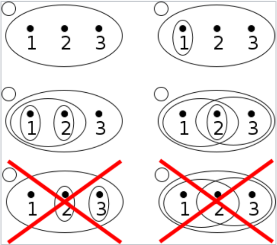
Well, the above definition sounds overly inclusive of many kinds of collections. Our understanding of topology will not be complete without a counter example. Here is a perfect example from this great Wikipedia article on Topological Spaces:

“Four examples and two non-examples of topologies on the three-point set ${1,2,3}$. The bottom-left example is not a topology because the union of ${2}$ and ${3}$ [i.e. ${2,3}$] is missing; the bottom-right example is not a topology because the intersection of ${1,2}$ and ${2,3}$ [i.e. ${2}$], is missing.” (ibid) If you want to see quickly what I see in this image, note that in the fourse examples on the top the unions and intersections of the subsets are present in the collection, but that some intersections or unions of elements are absent within the two at the bottom. More intuitively, refering back to the verbal definition I gave before, connections are missing from the two collections at the bottom. Note that in the case of the one at the bottom-left, a connection could have been made by means of a union operator and that in the case of the one at the bottom-right, a connection could have been made by means of an intersection operator.

In short, in order to represnt a configuration mathematically, connections between the elements of a set must be represented, using subsets of the original set; connections can be made by means of intersection and union operations on sets within a collection; the results of intersection and union operations can be the empty set or the original set, among other things; if a collection of such subsets is closed to these two operations, i.e. the results end up being within the collection, then the aforesaid collection is called a topology. Note that the two examples on the top are rather trivial in terms of the set of connections or the configuration that they represent. Also note that the two configurations in the middle represent two distinct configurations and that both of them can be regarded as topologies; and that they do not have to be the same.

Among other alterations, commens and annotations in the brackets are added by the author.

[**]Note that the set elements are typically referred to as points but that they can also be higher-dimensional data points or other mathematical objects.

[*] Note that we can refer to ‘a topology’ in a similar sense as to which we would refer to the geomrty of an object as ‘a geometry’

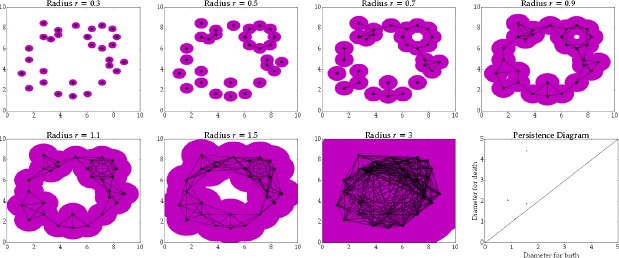
• Point-Set Topology (a.k.a. General Topology) What I described so far was General Topology, which is also known as Point-Set Topology. When it comes to the study of geometry, this sense of topology can be regarded as being concerned with the global properties of objects such as the number of connected components, the presence or absence of holes/handles (genera, the plural of genus), and answering questions such as whether the entire set resembles a doughnut, a double-doughnut, a disk, or a ball.

  

• Algebraic Topology (f.k.a. Combinatorial Topology) There is a more detailed (to the point/computational/combinatorial) view of topology that is mainly concerned with the structure of the connections between elements within [point]-sets. This latter sense of topology is widely known as Algebraic Topology.

Point-Set Topology: Point-Set topology, also called set-theoretic topology or general topology, is the study of the general abstract nature of continuity or “closeness” on spaces. Basic point-set topological notions are ones like continuity, dimension, and connectedness. 

In the context of Point Set Topology we discuss: Nodes, Arcs, Disks, Balls (topological models use to describe the space inside Point Neighbourhoods, Curves, Surfaces, and Solids) Loosely speaking, this sense of topology is evident in the global structure of a geometric model.

Algebraic Topology: Algebraic Topology, which includes Combinatorial Topology, is the study of “topological invariants” or ”topological properties” of combinatorial maps or decompositions of spaces such as [but not limited to] simplicial complexes.

In the context of Point Set Topology we discuss: Vertices, Edges, Faces, Bodies, (topological models used to tessellate/approximate/decompose Points, Curves, Surfaces, and Solids) Loosely speaking, this sense of topology is evident in the local structure of a geometric model.

We shall see how both of these senses come together in one equation describing topological invariants…: i.e. The Euler-Poincare Characteristic of discrete manifolds.