Rudiments of Linear Algebra & Computer Graphics

Introduction

This is a very short introduction for impatient Computer Graphics and Computational Design practitioners. Linear Algebra is a branch of mathematics. It is called linear algebra because it is the study of linear operators in an algebraic way (as opposed to, say, an arithmetic approach). Linearity is somewhat more twisted that you might think so we first explain what is meant by algebra.

Linear Algebra

Algebra

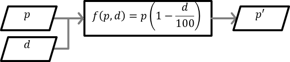
Suppose you are shopping for an item of clothing worth 14.99 bucks and that there is a discount percentage of 17.5 percent on it. To calculate the discount price you would find the 17.5 percent of 14.99 and subtract it from 14.99. This would be an arithmetic approach. Instead, if you generalize the problem and transcend the numbers to numerical variables (a.k.a. parameters or arguments), you can write: $$ \begin{equation} p'= p(1-\frac{1}{100}) \end{equation} $$ This formula is now working like a machine (a function) that maps the price of every item dubbed p with a discount percentage d, to a new discount price denoted as p'. Conceptually, this machince can be concieved as a black box with inputs and outputs (possibly more than one):

A function of some scalar variables in a set to a variable in some other set is often figuratively described as a map and is shown as $f:v↦w$ (read as function f that maps v to w), where the set v is referred to as the [input] domain and the set w is referred to as the [output] range (a.k.a. codomain) of the function in question.

def DiscountPrice(p,d):  
    p_prime=p*(1-d/100)  
    return p_prime

The keyword ‘def’ in Python marks a function definition. The keyword ‘return’ brings the imaginary cursor/calculator where it used to be, i.e. before calling th function and thus it effectively delivers the output[s] of the function.

Dimensionality

It might appear from the above definition that functions can only put out one variable at a time. However, we can easily generalize functions to take in and put out more than a single number. That is the essential reason to go to higher dimensions and define vectors, matices, and tensors. Although a geometric intuition (1D, 2D, and 3D) is often helpful to visualize multi-dimensionality, it can also be misleading. Dimensionality is a concept that has to do with combinations of (often numerical) elements from sets. $$ \begin{equation} \begin{cases} & \mathbb{R}^1=\mathbb{R} \text{ one dimensional vectors or scalars }\\
& \mathbb{R}^2=\mathbb{R}\times \mathbb{R}:={(x,y)|x\in \mathbb{R} \wedge y\in \mathbb{R}} \\
& \mathbb{R}^3=\mathbb{R}\times \mathbb{R}\times \mathbb{R} :={(x,y,z)|x\in \mathbb{R} \wedge y\in \mathbb{R} \wedge z\in \mathbb{R}} \\
\end{cases} \end{equation} $$

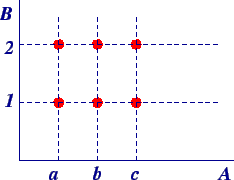
Have you every wondered what is the meaning of $\mathbb{R}^2$? We are not raising the set of real numbers to any power, that exponent actually means something completely different: it implies the effect of the Cartesian product of two sets $\mathbb{R}$ and $\mathbb{R}$. To understand what a Cartesian Product mean, consider the following example: given two sets $A={a,b,c}$ and $B={1,2,3}$, their Cartesian Product is denoted as $A\times B$ and is (by definition) equal to $A\times B={(𝑎,1), (𝑎,2), (𝑏,1), (𝑏,2), (𝑐,1), (𝑐,2)}$$

While it is customary to present the elements of a product set as tuples (pronounced like tewple, a generalization of double, triple, quadruple, quintuple, etc.), in Linear Algebra we often write such elements as vectors, most conventionally as ‘column vectors’ that look like this: $\mathbf{v}=[x,y,z]^T=\begin{bmatrix}x\\y\\z\end{bmatrix}\in \mathbb{R}^3$

where $T$ is not an exponent but the ‘transpose’ operator, which rewrites the matrix such that every row becomes a column and vice versa. multi-dimensionality is a concept best understood by means of the Cartesian product of sets. Although we can visualize 1D, 2D, and 3D spaces of numeric tuples, that we cannot conveniently visualize higher dimensional tuples does not mean that they are not understandable. Higher dimensional tuples are also tuples, but they are not necessarily related to relativity, quantum physics and sci-fi stories.

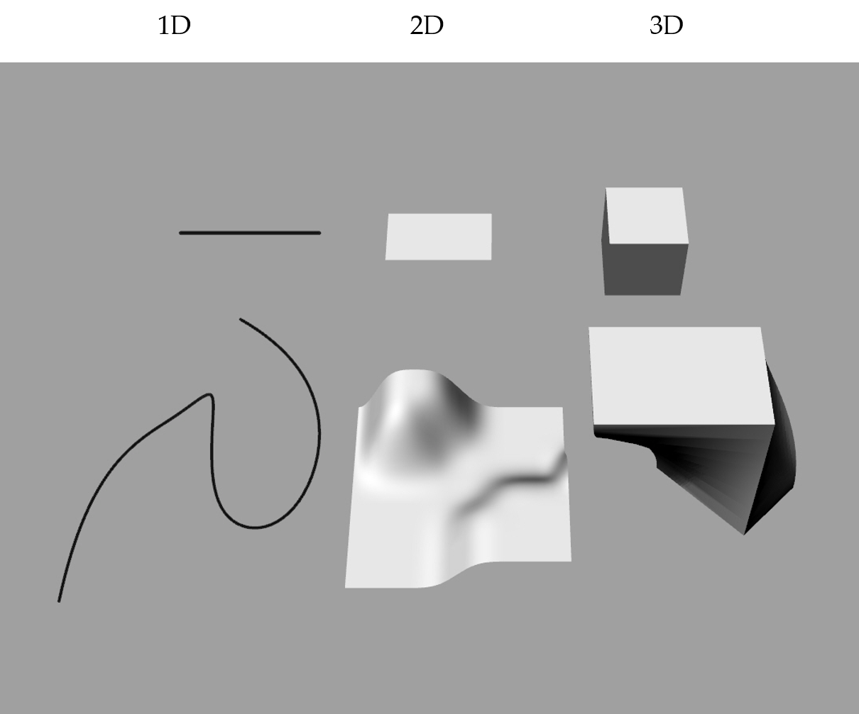
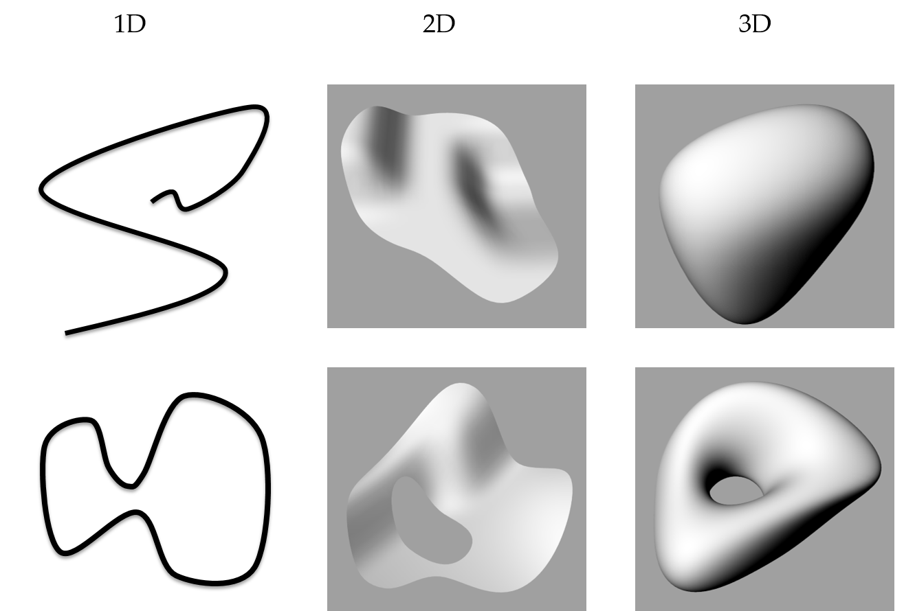
How would you appraise the dimensionality of the following objects? They all appear to be drawn in a 3D environment and yet there is something quite 1-dimensional about the first one from the left and something quite 2-dimensional about the one in the middle and so on.

In fact, when we say thet a curve is 1D, what we mean is that it is locally every-where similar to (topologically speaking, homeomorphic to) a Euclidean space of dimension 1, that is a line. Similarly, when we say a surface is 2D, we mean that it locally everywhere resembles a plane, that is a 2D Euclidean space. However, there are cases where objects cannot be considered locally smooth as such such as the curve of the leter x, which at the cross section cannot be considered being similar to a line. To distinguish spaces that have such smoothness from those that do not, we use the mathematical concept of a manifold, more specifically a d-manifold is an object that is locally every-where similar to a d-dimensional Euclidean space, i.e. $\mathbb{R}^d$:

Philosophically, the reason we call them manifolds is that their global shape is kind of folded and so their global look does not look linear, however they are everywhere locally linear.

• 0D: Point (the space therein everywhere resembles a 0-dimensional Euclidean Space)
• 1D: Curve (the space therein everywhere resembles a 1-dimensional Euclidean Space)
• 2D: Surface (the space therein everywhere resembles a 2-dimensional Euclidean Space)
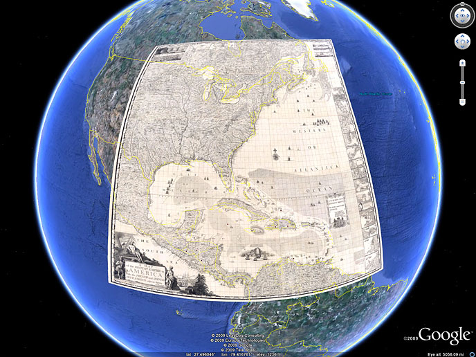
• 3D: Solid (the space therein everywhere resembles a 3-dimensional Euclidean Space)

  

  I hope the third definition rings a bell: have you ever wondered why for so long our ancestors used to think that the earth is flat? Well, it turns out that some people still do not believe that it is round and one of them is so persistent that wants to go into the space and check it out with his own rocket. Had our planet been like a donut, globally, we would have probably had the same assumptions about its flatness for ages as well.

  

  It seems that wherever we are, compared to our scale of life, the surface of the earth looks convincingly flat, regardless of the bumps, so it is only natural to draw geographical maps on rectangular surfaces. Therefore, a manifold conceptualization of the earth surface seems perfectly rational as it allows it to be both spherical globally and rectangular locally.

Linearity

In common language, linearity is about the linear dependency between two variables, phrases like the more of this the less of that and the more of this the more of that express linearity. In mathematical terms, there are a few senses of linearity of which one pertains to the case of Linear Algebra: Linear Maps. A function/map is said to be linear if it meets the following conditions: that the result of applying the function on a multiple of a variable is the same as multiplying the mapped variable by that same multiple and that the result of applying the function to the sum of two variables is the same as adding the mapped variables. In other words: $f(\alpha x)=\alpha f(x)$ and $ f(x+y)=f(x)+f(y)$ These conditions seem so strict that even a simple function like $f(x)=2x+1$, whose graph is a line, cannot be called linear (in fact this function is called an affine function, i.e. roughly speaking, a generalized category of linear functions). However, in more specific terms, i.e. in the context of Linear Algebra, when we speak of linearity, we are exactly talking about linear maps. In order to understand linear maps, firstly we need to understand what is meant by mapping. This brings us to the topic of matrices (plural form of matrix, also written as matrixes, though much less frequently). You can look at a matrix as a table full of numbers but what a matrix actually represents is a function of multiple input variables that results in multiple output variables. We shall see in more detail how such functions work but for now, consider the following operation: $m(\mathbf{x})=\mathbf{b}=\mathbf{A}\mathbf{x}$ in which a vector (a column tuple of scalars, a member of a Cartesian product of sets of scalars) is multiplied by a matrix and the result of this multiplication is another vector, probably in a different space. The reason we show vectors and matrices in bold roman letters is two avoid confusion between vectors (multi-dimensional points) and scalars (one-dimensional points or numbers). The most typical notation convention for Linear Algebra is to denote:

• scalars as lower-case Greek letters, preferably those that are distinct from Latin letters
• vectors as lower-case bold Latin letters, preferably using the last letters in the alphabet
• matrices as upper-case bold Latin letters, preferably using the first letters in the alphabet

We are running a bit forward and you are probably wondering why we did not mention anything about vectors being like arrows and so on. That story will come soon but believe it or not it is only a misconception about vectors. Be patient. You have most probably seen a matrix at least once in your life; so you know that it has columns and rows. You can consider each column as a vector, which immediately implies that every vector is a matrix as well. On the other hand, every row of a matrix can be considered as a transposed vector or a row-vector. For being absolutely clear about what matrices do, we can write down their dimensions as subscripts in the form of ‘number of rows’ $\times$ ‘number of columns’. In addition, we can also write down their ‘entries’ (the items within the matrix) in the form of $A_{i,j}$, indicating their locations addressed with a tuple of integers. Referring back to the so-called linear map defined above, we can rewrite it indicating dimensions:

• a note on notation: when we write matrix/vector entries, we do not use boldface letters because the entries are scalars, however, by denoting their multi-dimensional address we can see that they belong to a matrix or a vector. $$ \begin{equation} [b_{i}]_{m\times 1}=[A_{i,j}]_{m\times n}[x_j]_{n\times 1} \end{equation} $$ In other words, back to our very first definition of the vectors, it can be seen that the above operation takes in a vector from an n-dimensional space and puts out a vector from an m-dimensional space. This is exactly why it is called a map. Therefore, a matrix can be conceptualized as a mapper or simply called a map [function]. In mathematical terms, this is written as $\mathbf{A}\in \mathbb{R}^{m\times n}: \mathbf{x}\in \mathbb{R}^n \mapsto \mathbf{y}\in \mathbb{R}^m$. The same way a vector is a member of a Cartesian Product of sets, a matrix is said to be a member of a Cartesian Product of two multi-dimensional sets of m-tuples and n-tuples. What happens in the middle of the matrix and the vector on the right side is a matrix-matrix multiplication. A matrix-matrix multiplication is a result of multiple dot-products, which we will explain in the following sections. For now, it suffices to see the expansion of the matrix-matrix multiplication: $$ \begin{equation} [C_{i,j}]_{m\times n}=[A_{i,k}]_{m\times p}[B_{k,j}]_{p\times n} \end{equation} $$ where $$ \begin{equation} C_{i,j}=\sum_{k\in[0,p)} A_{i,k}B_{k,j} \end{equation} $$ Note that in the context of computation, indicies (plural form of index, means addresses of items within an array, stack, list, and alike) always start from 0. Now we are prepared to see the meaning of linearity in Linear Algebra: Maps represented by matrices operate by means of matrix-vector multiplication. and they are linear in the sense that they remain linear under the operation of addition and scalar multiplication respectively, meaning that if $f(\mathbf{u})\equiv \mathbf{A}\mathbf{u}$, then: $f(\mathbf{u}+\mathbf{v}) = f(\mathbf{u})+f(\mathbf{v})$ and $f(\alpha \mathbf{u}) = \alpha f(\mathbf{u})$, on the condition that the two vectors $\mathbf{u}$ and $\mathbf{v}$ are of the same dimension. This is because of the following identities: $$ \begin{equation} f(\mathbf{u}+\mathbf{v})=\mathbf{A}(\mathbf{u}+\mathbf{v})=\mathbf{A}\mathbf{u}+\mathbf{A}\mathbf{v}=f(\mathbf{u})+f(\mathbf{v}) \end{equation} $$ $$ \begin{equation} f(\alpha \mathbf{u})=\mathbf{A}(\alpha\mathbf{u})=\alpha\mathbf{A}\mathbf{u}=\alpha f(\mathbf{u}) \end{equation} $$

Vectors and their meaning

So far we presented vectors as tuples or column-matrices of scalars indicating points in higher dimensional spaces. You might be waiting for a geometric/intuitive definition. Even though geometric intuitions are mostly helpful for gaining a deeper understanding, they might also be harmful in case of bringing about false associations. For instance, associating vectors with arrows has the false association of a geometric shape of an arrow with the vector itself, which is nothing but a tuple of numbers. In particular, a vector, even if interpreted geometrically in a relatively low-dimensional space, does not have a location, let alone having a shape. It is only for our understanding that we sometimes draw arrows to understand what vectors do. What vectors do can be simply understood as giving directions in a multi-dimensional space. If you tell someone who is looking for an address to go forward towards the East for 100 steps and then turn left towards the North and continue forward for 200 steps, you are implying a direction in the form of $(right, up)=(100,200)$. Since we did not mention the location from which you gave this address/direction, it can be anywhere on the planet. In other words, all such directive addresses are represented with the same vector; and so, this vector does not have a location uniquely related to its information-content. In that sense, it is kind of wrong to show it with an arrow, unless we know what we mean by that: that any other arrow in the same direction and the same length/magnitude is equal to the arrow in question. 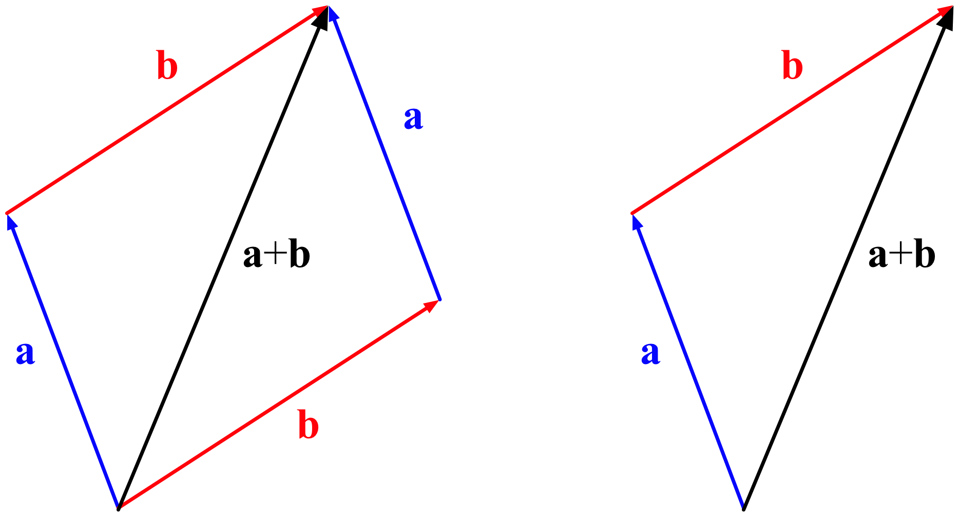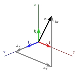You hopefully remember some things from your primary school maths books where geometry was taught by drawings. In that fashion, we can conceive vector operations as abstractions of some physical phenomena such as interactions of mechanical forces.

While such drawings may be interesting for getting an intuition, they do not directly give us clues as to how we can compute with vectors. In fact, there is a more modern version of geometry started by René Descartes, which is called Analytic Geometry, as it goes beyond such drawings and introduces a ‘coordinate system’, better known as the ‘Cartesian Coordinate System’:

The introduction of this coordinate system has revolutionized geometry, science, and engineering ever since. Taking the idea of vectors as directives/addresses, it can be seen in the above image that any vector can be considered to be the sum of any sequence of consecutive vectors in arbitrary directions such that the end of the first one becomes the beginning of the next one and so forth; therefore, if we choose a few important directions, called principal axes (plural of axis) we obtain a global system for describing components in terms of multiples of steps in the direction of such axes. If the vectors along such axes could also be represented in terms of vectors in other axes, then our attempt would be pointless. To ensure that this does not happen, it suffices to ensure that the so-called principal axes are ‘linearly independent’. i.e. once cannot obtain a vector along one axis as a ‘linear combination’ of vectors along other axes, where an expression in the following form is called a linear combination: $\mathbf{u}=\alpha_0\mathbf{e}_0+\alpha_1\mathbf{e}_1$. In higher dimensional contexts, it is customary to write principal vectors as $\mathbf{e}_k$; but in 3D, it is more convenient to denote principal vectors indicating the positive directions, respectively along the ${X,Y,Z}$ principal axes as $\mathbf{i}=[1,0,0]^T$, $\mathbf{j}=[0,1,0]^T$, and $\mathbf{k}=[0,0,1]^T$. In fact, these principal vectors bring about the concept of ‘dimension’, i.e. the very notion based on which we have expressed vectors so far as tuples or column-matrices. Besdies, we can perform vector additions not by drawing parallelograms but simple arithmetic operations, because if $\mathbf{u}=x_u\mathbf{i}+y_u\mathbf{j}+z_u\mathbf{k}$ and $\mathbf{v}=x_v\mathbf{i}+y_v\mathbf{j}+z_v\mathbf{k}$ then $\mathbf{u}+\mathbf{v}= (x_u+x_v)\mathbf{i}+(y_u+y_v)\mathbf{j}+(z_u+z_v)\mathbf{k}$.

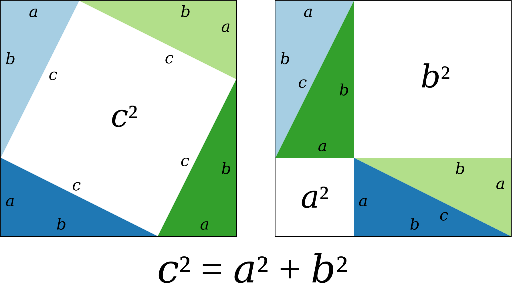
We spoke of the length or the magnitude of vectors but we did not mathematically represent them. In low-dimensional spaces, it is easy to check that the length of a vector can be computed using the Pythagoras theorem:“The sum of the areas of the two squares on the legs (a and b) of a right-triangle equals the area of the square on the hypotenuse (c)”.

$$ \begin{equation} \left | \mathbf{x} \right |=\left |[x_i]{n\times 1} \right |\equiv\left(\sum{i\in[0,n)}x_i^2\right)^{\frac{1}{2}} \end{equation} $$ In scientific contexts, this magnitude is called the ‘Euclidean norm’ of a vector, a function assigning a positive value to every vector in a vector space (and zero to the zero vector, i.e. $\left |\mathbf{0}\right |=0$). The Euclidean norm has the property that relates it to the so-called dot product of two vectors $\mathbf{x},\mathbf{y}\in \mathbb{R}^n$ shown as below:
$$ \begin{equation} \left \langle \mathbf{x},\mathbf{y} \right\rangle=\mathbf{x}.\mathbf{y}=\mathbf{x}^T\mathbf{y}\equiv\sum_{i\in[0,n)}x_iy_i \end{equation} $$ Therefore, the length/norm of a vector can be found from its dot product with itself:
$$ \begin{equation} \left | \mathbf{x} \right |=\left(\mathbf{x}^T\mathbf{x}\right)^{\frac{1}{2}} \end{equation} $$ Which in 3D space has a more familiar look:
$$ \begin{equation} \left | \mathbf{a} \right |=\left(a_x^2+a_y^2+a_z^2\right)^{\frac{1}{2}}= \sqrt{a_x^2+a_y^2+a_z^2} \end{equation} $$

Dot Product

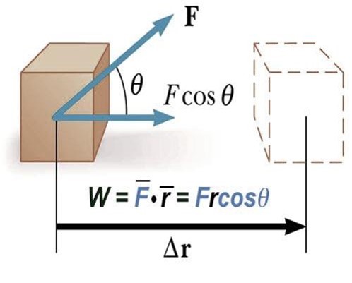
We have seen already one, and probably the most important, application of the dot product: finding the norm of a vector. In practice, the dot product of two vectors has many more applications such as detecting perpendicularity, measuring the degree to which two vectors are aligned in higher dimensions, measuring angles, computing flux of a vector field, etc. A very intuitive exemplary application of the dot product in physics is how work is calculated:

The work performed by a constant force vector along a straight linear displacement is equal to the dot product of the force vector and the displacement vector because it is largest when the two vectors are perfectly aligned, it is zero when they are perpendicular, and negative when they are in opposite directions. All of these is captured in the following: $$ \begin{equation} w=\mathbf{f}.\mathbf{d}=\left | \mathbf{f} \right |\left | \mathbf{d} \right |\cos(\theta) \end{equation} $$ Note that this equation means that work is a scalar quantity, which makes sense because you pay for work in cash, which does not have a direction! Now the question is, what does this equation have to do with the previous definition of the dot product given above? In other words, where does the cosine function come from?

To answer this question, we need to represent the two vectors in terms of the principal vectors. Without loss of generality, let us do this in a 2D Cartesian coordinate system:

$$ \begin{equation} \text{Let}; \mathbf{a}=\left | \mathbf{a} \right |\cos(\alpha)\mathbf{i}+\left | \mathbf{a} \right |\sin(\alpha)\mathbf{j} \end{equation} $$

$$ \begin{equation} \text{Let}; \mathbf{b}=\left | \mathbf{b} \right |\cos(\beta)\mathbf{i}+\left | \mathbf{a} \right |\sin(\beta)\mathbf{j} \end{equation} $$ and then the angle between the two vectors, previously called $\theta$ will be equal to $\theta=\beta-\alpha$

and so, by using our previous definition of the dot product:

$$ \begin{equation} \mathbf{a}.\mathbf{b}\equiv\left \langle \mathbf{x},\mathbf{y} \right\rangle=\mathbf{x}.\mathbf{y}=\mathbf{x}^T\mathbf{y}\equiv\sum_{i\in[0,n2)}x_iy_i=\left | \mathbf{a} \right |\cos(\alpha)\left | \mathbf{b} \right |\cos(\beta)+\left | \mathbf{a} \right |\sin(\alpha)\left | \mathbf{b} \right |\sin(\beta) \end{equation} $$ which can be simplified as: $$ \begin{equation} \mathbf{a}.\mathbf{b}=\left | \mathbf{a} \right |\cos(\alpha)\left | \mathbf{b} \right |\cos(\alpha)+\left | \mathbf{a} \right |\sin(\alpha)\left | \mathbf{b} \right |\sin(\beta)=\left | \mathbf{a} \right |\left | \mathbf{b} \right |\left(\cos(\alpha)\cos(\beta)+\sin(\alpha)\sin(\beta)\right) \end{equation} $$ which can be simplified even further using the famous trigonometric identity $\cos(\alpha \pm \beta) = \cos \alpha \cos \beta \mp \sin \alpha \sin \beta$: $$ \begin{equation} \mathbf{a}.\mathbf{b}=\left | \mathbf{a} \right |\cos(\alpha)\left | \mathbf{b} \right |\cos(\alpha)+\left | \mathbf{a} \right |\sin(\alpha)\left | \mathbf{b} \right |\sin(\beta)=\left | \mathbf{a} \right |\left | \mathbf{b} \right |\left(\cos(\beta-\alpha)\right)=\left | \mathbf{a} \right |\left | \mathbf{b} \right |\cos(\theta) \end{equation} $$

Cross Product

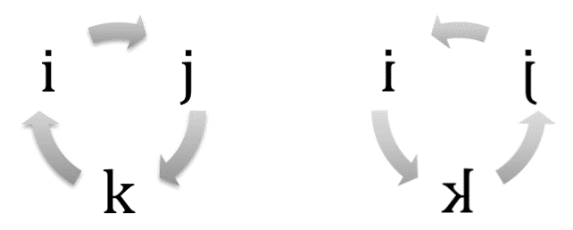
The cross product of two vectors is a vector perpendicular to both of them and thus perpendicular to the plane ‘spanned’ by the two vectors in question, and is equal in magnitude to the norms of the two multiplied by the sine of the angle in between them. As opposed to the dot product, the cross product is non-commutative, i.e. it matters which vector comes first and which one second. In fact $\mathbf{a}\times\mathbf{b}=-\mathbf{b}\times\mathbf{a}$. Let us take an intuitive approach to finding out the cross product of two vectors, based on the cross product of the principal vectors according to the initial definition:

$$ \begin{equation} \mathbf{i}\times\mathbf{j}=\mathbf{k};; \text{and};; \mathbf{j}\times\mathbf{i}=-\mathbf{k} \end{equation} $$

$$ \begin{equation} \mathbf{j}\times\mathbf{k}=\mathbf{i};; \text{and};; \mathbf{k}\times\mathbf{j}=-\mathbf{i} \end{equation} $$

$$ \begin{equation} \mathbf{k}\times\mathbf{i}=\mathbf{j};; \text{and};; \mathbf{i}\times\mathbf{k}=-\mathbf{j} \end{equation} $$ and so as a mnemonic, we can keep these pictures in mind:

and so, the cross product of two vectors $\mathbf{a}=a_x\mathbf{i}+a_y\mathbf{j}+a_z\mathbf{k}$ and $\mathbf{b}=b_x\mathbf{i}+b_y\mathbf{j}+b_z\mathbf{k}$ will be:

$$ \begin{equation} \mathbf{a}\times\mathbf{b} = (a_x\mathbf{i}+a_y\mathbf{j}+a_z\mathbf{k})\times (b_x\mathbf{i}+b_y\mathbf{j}+b_z\mathbf{k})=(a_yb_z-a_zb_y)\times \mathbf{i}-(a_xb_z-a_zb_x) \times \mathbf{j}+(a_xb_y-a_yb_x) \times \mathbf{k} \end{equation} $$

and because it is such a long equation to remember, we often use a determinant notation as a mnemonic (even though it is not exactly a matrix determinant):

$$ \begin{equation} \mathbf{a}\times\mathbf{b} = (a_x\mathbf{i}+a_y\mathbf{j}+a_z\mathbf{k})\times (b_x\mathbf{i}+b_y\mathbf{j}+b_z\mathbf{k})= \begin{vmatrix} a_y & a_z\b_y & b_z \end{vmatrix} \mathbf{i}-\begin{vmatrix} a_x & a_z\b_x & b_z \end{vmatrix} \mathbf{j}+\begin{vmatrix} a_x & a_y\b_x & b_y \end{vmatrix} \mathbf{k}\equiv \begin{vmatrix} \mathbf{i} & \mathbf{j} & \mathbf{k}\a_x & a_y & a_z\b_x & b_y & b_z\end{vmatrix} \end{equation} $$ Before talking about the magnitude of the cross product, let us get more comfortable with them and see how they can be used to make planes. Planes will be introduced in more detail later but for now, it suffices to think of them as infinitely large ellipsoids or rectangles with two opposite sides called front and back, characterized by a vector perpendicular to them, that which is called a ‘normal vector’, sometimes briefly called a ‘normal’.

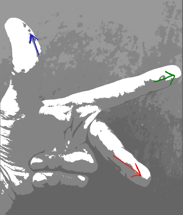
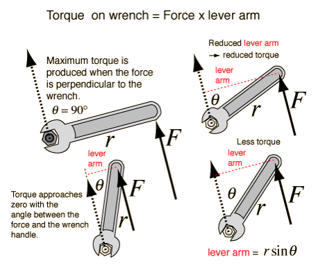
To remember how to determine the direction of the cross product of two vectors, I show you a trick with my left hand: if you fix your left hand as a little XYZ gizmo, if putting your middle finger aligned with the first vector, and putting your index finger aligned with the second vector, then your thumb will show you the direction of the cross-product of the two. These three fingers are respectively marked with RGB (Red,Green,Blue) arrows as is conventional.

Now, let us see the magnitude of the cross product in the context of a physical example: torque.

In the above image, you can see that the amount of torque (which could be conceived as ‘rotational force’, in a manner of speaking) is a vector quantity (because it has a direction/orientation) which is the kind of force that can cause rotary/angular acceleration without displacing the object axially. When trying to loosen a rusty nut with a wrench, you need to turn the wrench counter-clockwise hard so the nut ‘goes out’ along the bolt; and when trying to tighten a nut on a rusty bolt, you need to turn the wrench hard in the clockwise direction so that the nut ‘goes in’. This is something you can easily remember with a right-hand trick: if you wrap your four fingers scanning the angle between the two vectors from the first towards the second, then your thumb will show the direction of the cross product (e.g. torque).

Mathematically, the amount of torque depends obviously on the amount of force applied; but not only that: it also depends on the size of the wrench, or actually the distance from the center of the bolt/nut to the point on which you apply the force. Note that if you apply the force parallel to the wrench, you either take it off the bolt/nut or do nothing effective. For the force to be maximally effective it needs to be applied perpendicular to the wrench. You can imagine that there must be a smooth transition of effectiveness between these two extremes,i.e. in other angles, and that is exactly what the sine function does:

$$ \begin{equation} \left | \mathbf{a}\times\mathbf{b}\right | = \left | \mathbf{a}\right |\left | \mathbf{b}\right |\sin(\theta) \end{equation} $$

Planes and their meaning

I already gave a loose definition of planes while explaining the primary purpose of the cross-product. You might be wondering, however, why on earth would we need to make a plane? Is it not so that there is a global plane XY whose normal is the Z-axis? In practice, take my words, when creating a 3D object you want to place it on a plane, rather than merely on a point. In fact, a single point does not have any orientation, so it does not give us enough clues as to how we should actually place something. So, make it a rule of thumb that we should ‘place things on planes’. The reason to do this is that to place things unambiguously in 3D space, one needs to know their orientation as well as their [center/corner] position. Look at your right hand and grab an imaginary axis as a rotation axis. The direction along which you wrapped your fingers, the counter-clockwise direction is by convention considered as the positive trigonometric direction. In addition to knowing what the ground under an object looks like (a plane surface), you also need to know which side of it is front and which side is back. This is determined by the normal vector. In the example explained here this is the direction your right thumb is pointing to; and the plane in question is the plane on which the rotation happens. 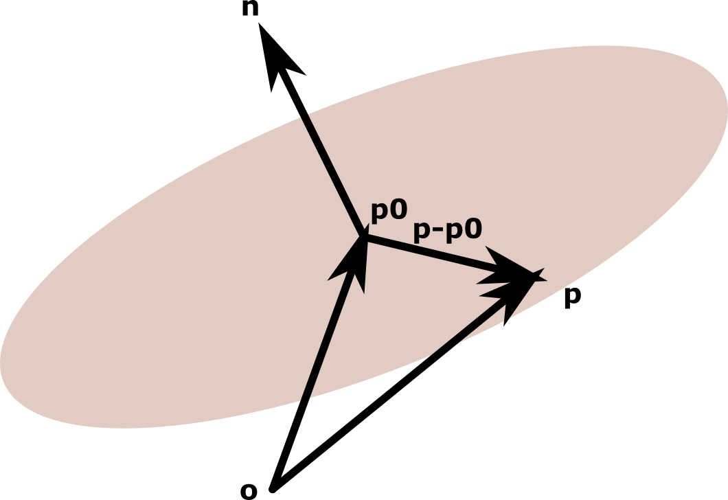Philosophically, there are multiple ways to make planes, from three points, from a normal vector and a point to be considered as an origin. Let us consider the latter first and see if it is equal or unequal to the former in terms of information content. Suppose we are given a vector $\mathbf{n}=[a,b,c]^T$, it is desired to find a plane perpendicular to this vector, which includes the point $\mathbf{p}=[x,y,z]^T$. Here I open two parentheses to explain an important point:

• what is the difference between points and vectors? In fact, in terms of information content points and vectors are kind of the same. It is the way of interpretation that makes them different from another. When we are reading a vector that is called a point, we consider that vector to be a ‘position vector’, i.e. a vector drawn from the origin $\mathbf{p}_0=[x_0,y_0,z_0]^T$ or another point considered to be their origin, towards the point in question. In other words, vectors can be assumed to be indicating the displacement (from anywhere to anywhere, they are not tied to any location) and point to be representing positions measured from the origin. Note that based on this distinction, a point can only be a point in the context of a known plane. A single point in the context of two different planes will point to two different positions, because it is in fact merely a vector drawn from an origin, the question is which origin(, and also moving along which axes, reflect on this a little).

For finding the plane in the above question, I should like to give you a more formal definition of a plane as a ‘locus’ (a location/region in space whose constituent points are characterized mathematically, a.k.a. the mathematical location) of points whose position vectors drawn from a point considered to be the origin is perpendicular to a vector considered to be normal to that plane, i.e. pointing unambiguously towards the front side of it.

To write this down mathematically, we use an important property of dot product of two vectors that says two vectors are perpendicular to each other ‘if and only if’ their dot product is zero. The phrase ‘if and only if’ indicates a ‘necessary & sufficient’ condition, i.e. a logical statement that can be read in both directions:

• if the dot product of two vectors is zero, we can conclude that they are perpendicular
• if two vectors are perpendicular their dot product has to be zero

So, by denoting everything mathematically: $$ \begin{equation} \left( \mathbf{p}-\mathbf{p}_0 \right).\mathbf{n}=0 \end{equation} $$ Note that since both vectors $\mathbf{p}$ and $\mathbf{p}_0$ are not yet written in the coordinate system of the desired plane, they are both indicating points from a global origin assumed/implied to be $\mathbf{O}=[0,0,0]^T$; and thus the position vector on the desired plane, when added to $\mathbf{p}_0$ will be equal to $\mathbf{p}$. Draw this to understand it.

$$ \begin{equation} \begin{bmatrix}x\ y\z\end{bmatrix}-\begin{bmatrix}x_0\ y_0\z_0\end{bmatrix}.\begin{bmatrix}a\ b\c\end{bmatrix}=0 \Rightarrow a(x-x_0)+b((y-y_0)+c(z-z_0)=0 \Rightarrow ax+by+cz=ax_0+by_0+cz_0 \end{equation} $$

Well, as you see, we have obtained an equation that characterizes a typical point on the desired plane, this is the plane equation as a locus that we were after.

Now, consider the two ways I mentioned for making planes: from three points or from a point and a normal vector. We just went through the process of making the latter. Without going into much details let me show you right away that a given point in the plane characterized with three points has a more informative location. That is because such a plane not only would have an orientation determined by a normal vector, but also could we write down coordinates for any point on this plance along two axis vectors. These axis vectors are not present in the plane we described mathematically so far.

Suppose we are given the three points $\mathbf{p}_0=[x_0,y_0,z_0]^T$, $\mathbf{p}_1=[x_1,y_1,z_1]^T$, and $\mathbf{p}_2=[x_2,y_2,z_2]^T$, and that it is desired to find the plane equation passing through these points. One way to think about this is to find a cross-product of two vectors $\mathbf{u}=\mathbf{p}_1-\mathbf{p}_0$ and $\mathbf{v}=\mathbf{p}_2-\mathbf{p}_0$, consider it as a normal vector and do the rest as we did before, but in doing so we shall loose some information regarding the axes of the plane in question. Instead, we can describe a typical on this plane as a linear combination of the two vectors $\mathbf{u}$ and $\mathbf{v}$:

$$ \begin{equation} \mathbf{p}=\mathbf{p}_0+s\mathbf{u}+t\mathbf{v} \end{equation} $$ where $s$ and $t$ are two scalar parameters determining the location of the typical point $\mathbf{p}$ unambiguously, provided the cross-product of the two vectors is not zero. This is why such vectors are said to have a span, i.e. a region of four quadrants, each of which looks like a rhombus/diamond. Again, there is a necessary and sufficient condition about vectors in 3D that two vectors are perfectly-aligned/parallel (but not necessarily of the same length) if and only if their cross-product is zero, in which case they cannot span any 2-dimensional plane region in 3D.